
Creep testing shows how a material responds to a static load and how it recovers once that load is removed. Combined with Time–Temperature Superposition (TTS), short tests at several temperatures predict long-term behavior. This study applies both to polypropylene.
- PP was held under a static stress of 5 × 10⁶ N/m² for 1800 s, then allowed 1800 s to recover
- Creep was measured from 15 °C to 95 °C in 5 °C steps; creep increased as temperature rose
- A master curve was built at a 20 °C reference temperature, with WLF and Arrhenius coefficients
- Run on the Alpha Metravib DMA+1000 with the built-in TTS function in Dyna+ software
Creep as a Window Into Long-Term Behavior
Creep is one of the most fundamental and dominant analytical tools used to study material behavior. These measurements help characterize the response of materials to a static load and their behavior once the same static load is removed.
Creep tests can be utilized in two ways: (1) to obtain fundamental information about a polymer, or (2) to investigate the material response under real, application-relevant conditions. These measurements can provide useful information about a material, such as relaxation time or permanent deformation. From an application point of view, the ability to create stable materials can be evaluated using creep measurements.
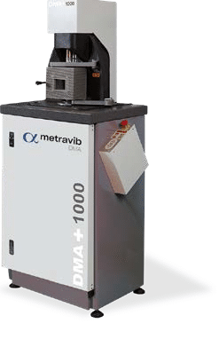
Figure 1. Alpha Metravib DMA
Moreover, creep measurements performed at different temperatures can be used to estimate the aging behavior of a material. This aging estimation can be carried out using the in-built Dyna+ software function known as TTS (Time–Temperature Superposition). This function allows the construction of time–temperature master curves by selecting a reference temperature. The master curve building process is explained in the application note titled “Building Frequency Temperature Superposition Master Curves.”
This creep study was performed on PP (polypropylene) using the Alpha Metravib DMA+1000.
Polypropylene in Tension From 15 °C to 95 °C
PP is characterized by its high toughness, rigidity, and crystalline nature, and is commonly used in industrial applications such as piping systems. The dimensions (h × b × t) of the specimen used for this study were 6.5 × 19.3 × 2.9 mm, respectively. The specimens were tested in tension mode (Figure 2).
A static stress of 5 × 10⁶ N/m² was applied for 1800 seconds, with a maximum displacement of 0.005 m. This static loading step was followed by a recovery period of 1800 seconds.
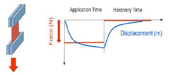
Figure 2. Tension mode
Since the objective was to study creep behavior together with TTS, creep measurements were performed at several temperatures ranging from 15 °C to 95 °C, with a stabilization time of 15 minutes at each temperature. The test parameters are summarized in Table 1.
Table 1. Test parameters
| Parameter | Setting |
|---|---|
| Static stress (N/m²) | 5 × 10⁶ |
| Duration (s) | 1800 |
| Temperature (°C) | 15 to 95, in 5 °C steps |
| Stabilization time at each temperature (min) | 15 |
| DMA | DMA+1000 |
| Test mode | Tension |
Creep Rises With Temperature
Figure 3 shows the static displacement obtained as a result of the applied static force at different temperatures from 15 °C to 95 °C. It can be observed that applying the static force for 1800 seconds was sufficient to reach displacement stabilization, except at the highest temperatures used in the measurements. Similarly, the recovery time of 1800 seconds was also sufficient.
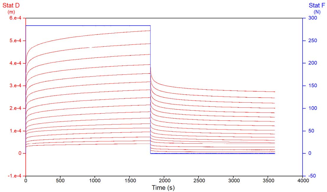
Figure 3. Static displacement under load and during recovery, 15 °C to 95 °C
Temperature is one of the most important variables, as most materials exhibit significantly different behavior below and above their glass transition temperature. Lowering the temperature reduces the mobility of polymer chains, leading to a decrease in free volume and, consequently, a reduction in creep [1,2]. This temperature effect can be clearly observed in Figure 3.
A Master Curve at 20 °C
Creep data collected at several temperatures were used to construct a master curve at a reference temperature of 20 °C. This master curve makes it possible to predict the creep behavior of the material at the reference temperature over a very long time scale. Master curve calculations were performed using both WLF and Arrhenius theories, and the corresponding coefficients are shown in Figure 4.
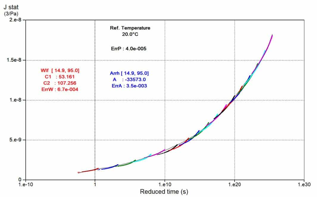
Figure 4. Creep master curve at 20 °C reference temperature, with WLF and Arrhenius coefficients
This TTS application enables analysis of creep behavior over several decades of time. This TTS module is particularly useful when limited experimental time is available but long-term material behavior is required.
What the Data Shows
This study demonstrates the capability of the DMA+1000 to perform creep measurements in combination with its in-built, user-friendly software functions for calculating and plotting master curves. The study successfully enabled the calculation and construction of a master curve at a reference temperature of 20 °C, as well as the determination of WLF and Arrhenius coefficients.
The bottom line
By combining creep testing with TTS, long-term material behavior can be predicted from short-term experiments, providing an efficient approach to evaluating aging and stability with the Alpha Metravib DMA+1000.
Creep and Time–Temperature Superposition
Get the complete application note, including all figures and test details, as a PDF.
Introduction to Dynamic Mechanical Analysis for Rubber Materials
How rubber engineers evaluate real-world material behavior. Inside the guide: guidance for improving analysis quality and useful direction for integrating DMA into research, development, and testing workflows.
1. Kevin P. Menard. Dynamic Mechanical Analysis: A Practical Introduction.
2. C. Macosko. Rheology: Principles, Measurements and Applications. VCH, New York, pp. 119–121.